Scotty 3D: A 3D Graphics Software Package

This is a course project for (CMU 15-662: Computer Graphics)[http://15462.courses.cs.cmu.edu/spring2023/].

This projects has four major modules impleemnetd. Each module taks me roughly 3 weeks to complete on average. The following sections will showcase the visual results I achieved after one module is completed. More details about the algorithms and methodologies will be added in the future.

Module 1: Rasterizer

Modern GPUs implement an abstraction called the Rasterization Pipeline. This abstraction breaks the process of converting 3D triangles into 2D pixels into several highly-parallel stages, allowing for a variety of efficient hardware implementations. In this assignment, you will be implementing parts of a simplified rasterization pipeline in software. Though simplified, your pipeline will be sufficient to allow Scotty3D to create preview renders without a GPU!

Different graphics APIs may present this pipeline in different ways, but the core steps remains consistent: a GPU draws things by running code (in parallel) on a list of vertices to produce homogeneous screen positions (+ extra varying data), building triangles from that list of vertices, clipping the triangles to remove parts not visible on the screen, performing a division to compute screen positions, computing a list of "fragments" covered by those triangles, running code on each fragment, and composing the results into a framebuffer.

Module 2: Mesh Editor

In this module, I wrote code to support the interactive editing of meshes in Scotty3D. Scotty3D stores and manipulates meshes using a halfedge mesh structure -- a local connectivity description which allows for fast local topology changes and has clear storage locations for data associated with vertices, edges, faces, and face-corners (/edge-sides).

Halfedges store the bulk of the connectivity information. They store a reference to the halfedge on the other side of their edge in Halfedge::twin, a reference to the halfedge that follows them in their current face in Halfedge::next, a reference to the vertex they leave in Halfedge::vertex, a reference to the edge they border in Halfedge::edge, and a reference to the face they circulate in Halfedge::face:

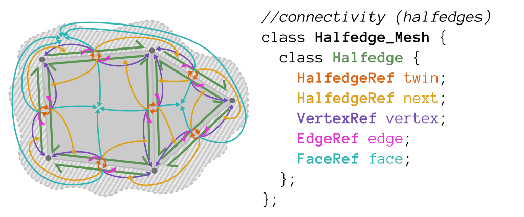
There are many mesh edit operations that were implemented in this module. Here are some examples: two for each of local operations and global operations.

Local::erase_vertex

Local::erase_edge

Global::loop_subdivide

Global::simplify

Module 3: Ray Tracer

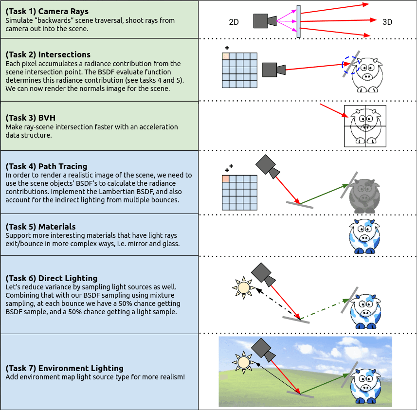
There are many sub-routeines in this module as shown in Fig-3. Detailed discussions follow.

Camera Rays

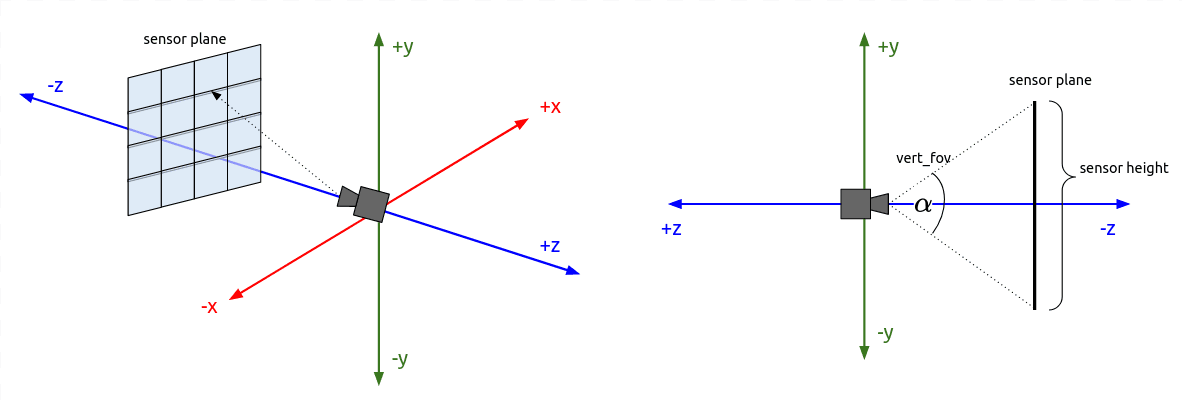
"Camera rays" emanate from the camera and measure the amount of scene radiance that reaches a point on the camera's sensor plane. (Given a point on the virtual sensor plane, there is a corresponding camera ray that is traced into the scene.) Your job is to generate these rays, which is the first step in the raytracing procedure.

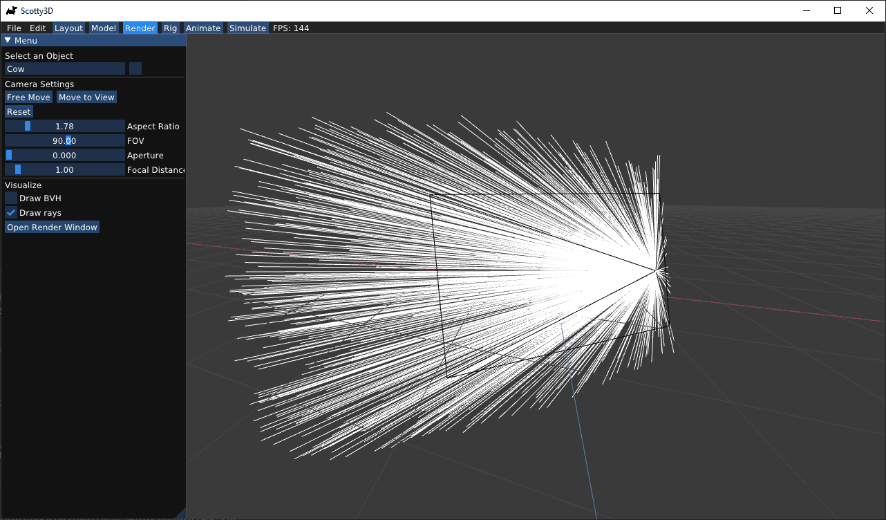
Visualized camera rays:

Intersections

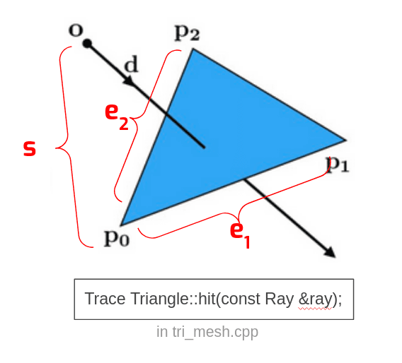
The first intersect routine you will implement is the hit routine for triangle meshes:

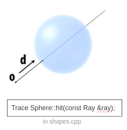
The second intersect routine you will implement is the hit routine for spheres:

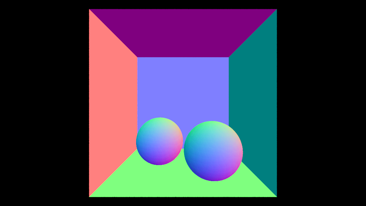
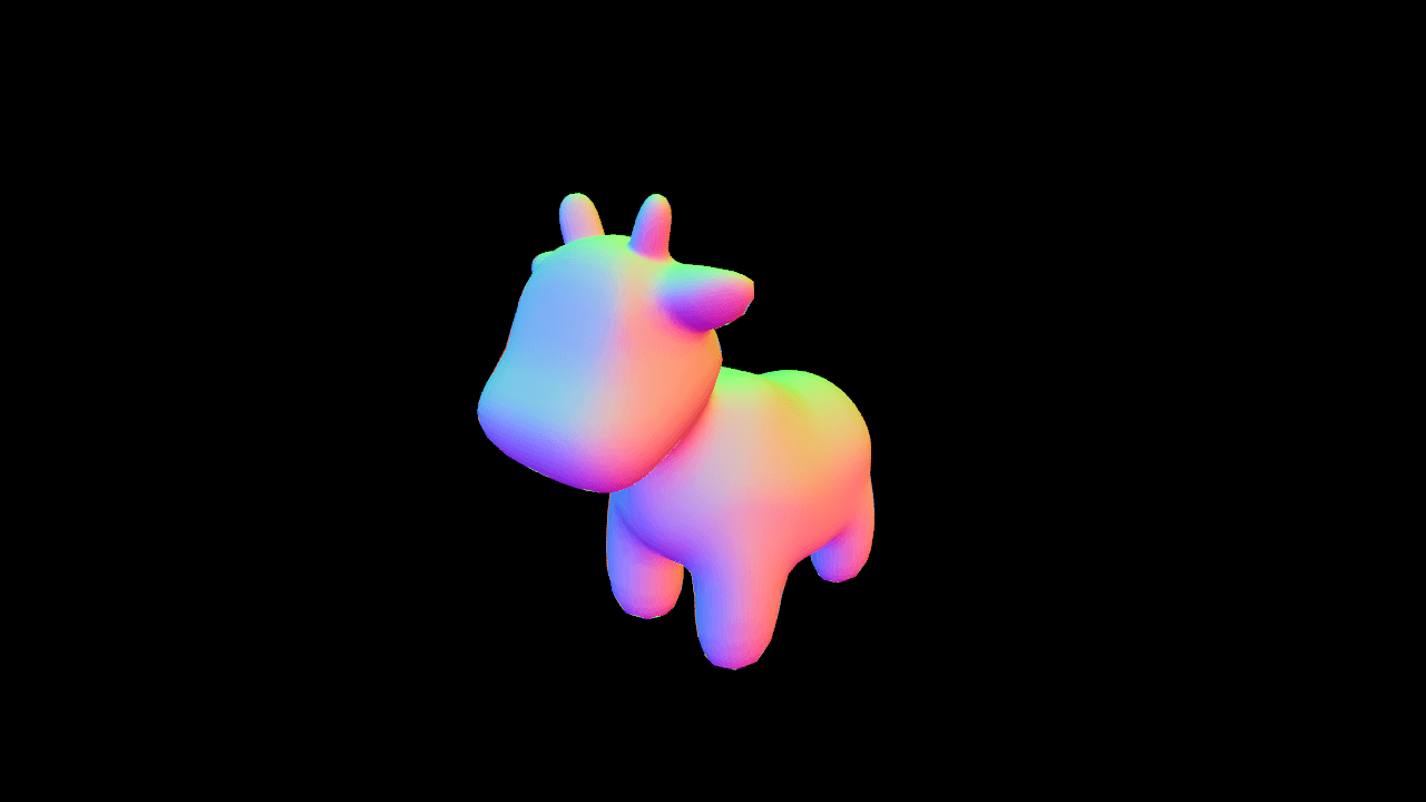
Results:

Path Tracing

Up to this point, our renderer has only computed object visibility using ray tracing. Now, we will simulate the complicated paths that light can take throughout the scene, bouncing off many surfaces before eventually reaching the camera. Simulating this multi-bounce light is referred to as global illumination, and it is critical for producing realistic images, especially when specular surfaces are present.

Implementation setps:

1. Lambertian
2. Sample indirect lighting
3. Sample direct lighting

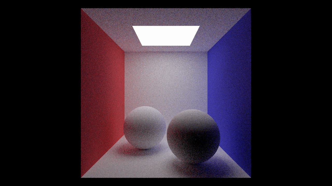
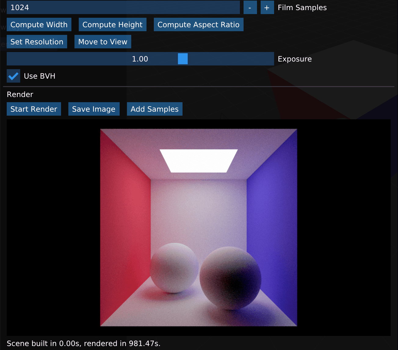
Reference images below show the time-quality tradeoff on an Intel Core i7-8086K (max ray depth 8). The second from the last image was rendered with a sample rate of 1024 camera rays per pixel and a max ray depth of 8. This will produce a relatively high quality result, but will take quite some time to render.

Materials

Now that we have implemented the ability to sample more complex light paths, it's time to add support for more types of materials. In this task you will add support for two types of specular materials: mirrors and glass.

Implementation setps:

1. Materials::Mirror
2. Materials::Refract
3. Materials::Glass

Direct Lighting

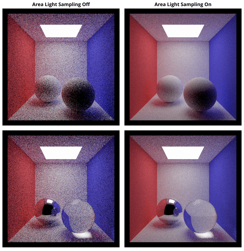
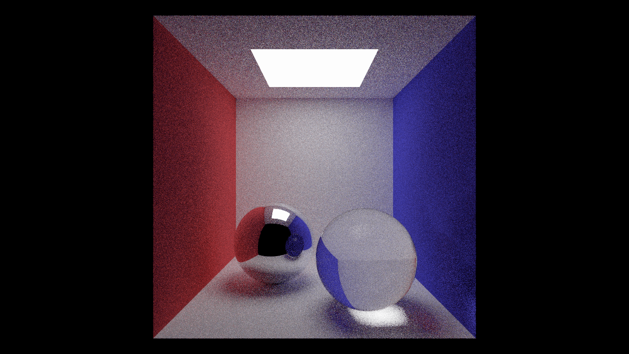
In this sub-routine, we will modify the sampling algorithm by splitting samples between BSDF scatters and the surface of area lights, a procedure commonly known as next event estimation.

First consider why sampling lights is useful. Currently, we are only importance sampling the BSDF term of the rendering equation (in which we have included the cosine term). However, each sample we take will also be multiplied by incoming radiance. If we could somehow sample the full product, our monte carlo estimator would exhibit far lower variance. Sampling lights is one way to importance sample incoming radiance, but there are some caveats.

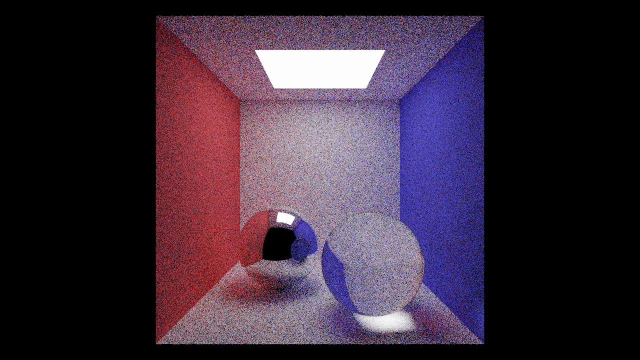
My results:

Environment Lighting

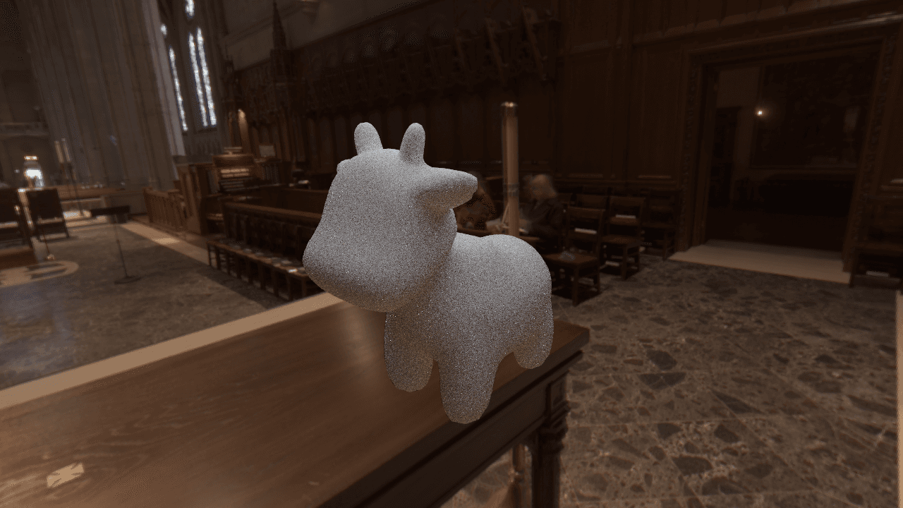
The final task of this assignment will be to implement a new type of light source: an infinite environment light. An environment light is a light that supplies incident radiance from all directions on the sphere. Rather than using a predefined collection of explicit lights, an environment light is a capture of the actual incoming light from some real-world scene; rendering using environment lighting can be quite striking.

My result:

Module 4: Animation System

This module completes Scotty3D's animation system, including skeletal animation, linear-blend skinning, and a particle simulation.

One of my cursory "art work" after this module is impleemnetd:

Spline Interpolation

Data points in time can be interpolated by constructing an approximating piecewise polynomial or spline. In this sub-routine we will implement a particular kind of spline, called a Catmull-Rom spline. A Catmull-Rom spline is a piecewise cubic spline defined purely in terms of the points it interpolates. It is a popular choice in animation systems, because the animator does not need to define additional data like tangents, etc.

Result:

Skeleton Kinematics

A Skeleton (declared in src/scene/skeleton.h, defined in src/scene/skeleton.cpp) is what we use to drive our animation. We can think of them like the set of bones we have in our own bodies and joints that connect these bones. For convenience, we have merged the bones and joints into the Bone class which holds the orientation of the bone relative to its parent as Euler angles (Bone::pose), and an extent that specifies where its child bones start. Each Skinned_Mesh has an associated Skeleton class which holds a rooted tree of Boness, where each Bone can have an arbitrary number of children.

Forward Kinematics

Result:

Inverse Kinematics

Result:

Linear Blend Skinning

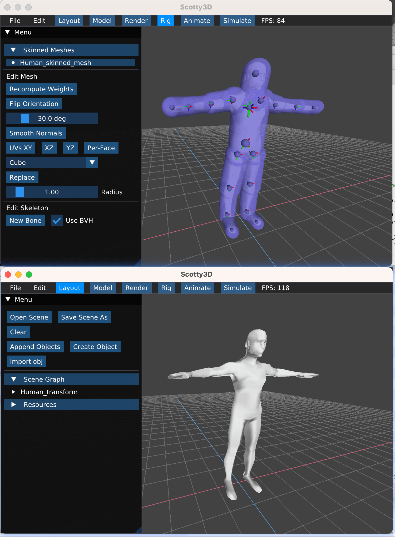
Now that we have a skeleton set up, we need to link the skeleton to the mesh in order to get the mesh to follow the movements of the skeleton. We will implement linear blend skinning using Skeleton::skin, which uses weights stored on a mesh by Skeleton::assign_bone_weights, which in turn uses the helper Skeleton::closest_point_on_line_segment.

Result (rig on the top and skinned model on the bottom):

Particle Systems

A particle system in Scotty3D is a collection of non-self-interacting, physics-simulated, spherical particles that interact with the rest of the scene. Take a look at the [slightly outdated] user guide for an overview of how to create and manage them.

Result:

Summary and Future Improvements